Modelling Financial Growth
Extends a simple exponential growth model to sequences of financial prices. A model of normally distributed logarithmic returns is demonstrated.
When we model the growth of a financial asset we are interested in its growth as a function of time. If we have a principal, ![]() , at time zero, what will its value be at time, t; what is the function p(t)? It is often natural to start with exponential growth as this works well for systems that do not grow fast enough to consume all the resources needed for growth. The main idea of exponential growth, however, is that there is a constant rate, r, of growth. The formula for p(t) is then derived from a simple differential formula:
, at time zero, what will its value be at time, t; what is the function p(t)? It is often natural to start with exponential growth as this works well for systems that do not grow fast enough to consume all the resources needed for growth. The main idea of exponential growth, however, is that there is a constant rate, r, of growth. The formula for p(t) is then derived from a simple differential formula:

where r is the constant rate of growth.
Solving this by integrating, we get:

![]()
where ![]() is taken to be 0, and
is taken to be 0, and ![]() is the starting principal.
is the starting principal.
Taking exponents

Thus
![]()
r here is a logarithmic return. To convert it to a decimal return, dr, we take the exponent and subtract 1.
![]()
And to convert the decimal return to a logarithmic return:
![]()
Substituting this value into the equation for p(t), we get the standard formula for compound growth.
![]()
Now suppose that we have a sequence of prices. We can compute the logarithmic returns for each interval in the series.
![]()
The log prices are
![]()
The log returns of this series are simply the sequential differences of log prices at a unit interval, in our example daily.
![]()
or equivalently.

The sum of the series of returns now is the same as the return over the whole interval since all but the first and last log prices cancel out:
![]()
The average log return over all the prices becomes:

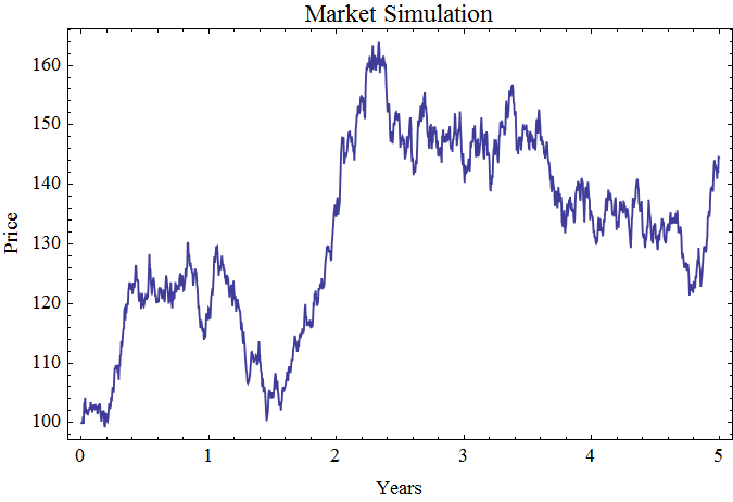
Now we have set up a structure to study the variability of market prices. If we take a sequence of prices, typically determined at the end of a market day. We can calculate the log returns for each interval. These log returns could be imagined as random variables as Louis Bachelier proposed in 1900. His thesis suggested that Brownian motion could be used to model stock market options. Let’s try modeling market log returns as behaving as normally distributed random variables. The graph below assumes 250 trading days in a year, with an expected annual gain of 7% per year, with a daily log return standard deviation of 0.01. The starting price is 100 and the series of log returns are accumulated after adding them to a starting point of log[100], creating a sequence of log prices. The exponent to base e is taken to convert to prices.

Superficially the model looks convincing, but we will show in subsequent notebooks that the normal distribution and Brownian motion are not a good choice to model market prices. We will use the methods described here as the basic frame work to examine stock market price time-series.
© Copyright 2013 Robert H. Rimmer, Jr. Sun 27 Oct 2013