Market Return Distribution
Looks at the time-series of the S&P 500 index since 1950 and examines nature of the distribution of log returns for this sequence. Including a stable distribution fit and the distribution tail behavior.
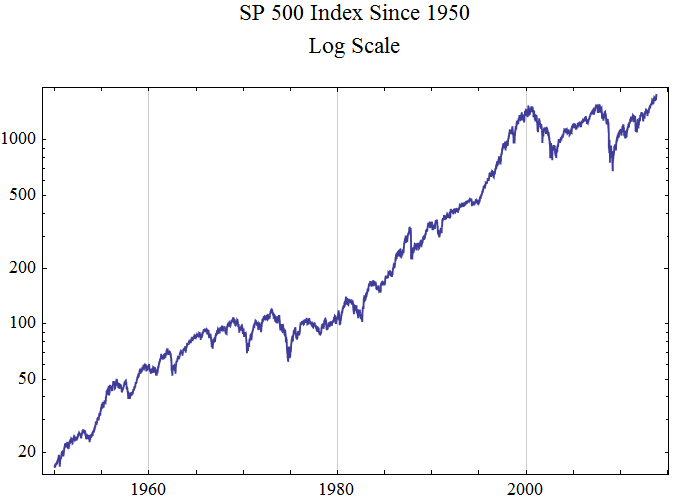
The graph below shows the daily closing SP 500 index on a logarithmic scale, since 1950.
Start ... Tuesday 3 January 1950
End ... Friday 25 October 2013

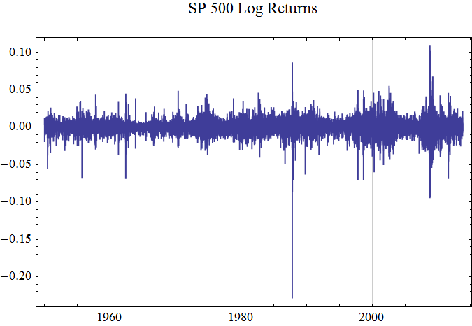
We can now easily calculate the market day log returns, by taking the sequential differences of the log index prices. The graph shows periodic clustering of high and low returns, suggesting that the log return process is not completely independent.
The histogram of the log returns shows a unimodal distribution with significantly greater kurtosis than a normal distribution, the fit of which is shown in green.
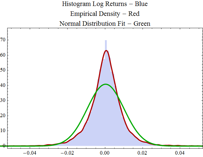
The Jarque-Bera test shows that the probability that the log return data come from a normal distribution is virtually zero.
| Statistic | P-Value | |
| Jarque-Bera ALM | 515278. | 6.021321249.519292941290667*^-111892 |
Financial Distribution Tail Behavior
The plot below shows a plot of the empirical distribution function, EDF, of minus x in blue, and 1-EDF[x], in red. Probability or 1- Probability for the right tail is on the ordinate axis and absolute value of x is on the abscissa. For comparison the fitted normal distribution tail is shown in green. The data tails are extremely heavy compared to the data tails of a normal distribution. The data tails also tend to become somewhat linear in the log log plot suggesting a Pareto tail behavior.
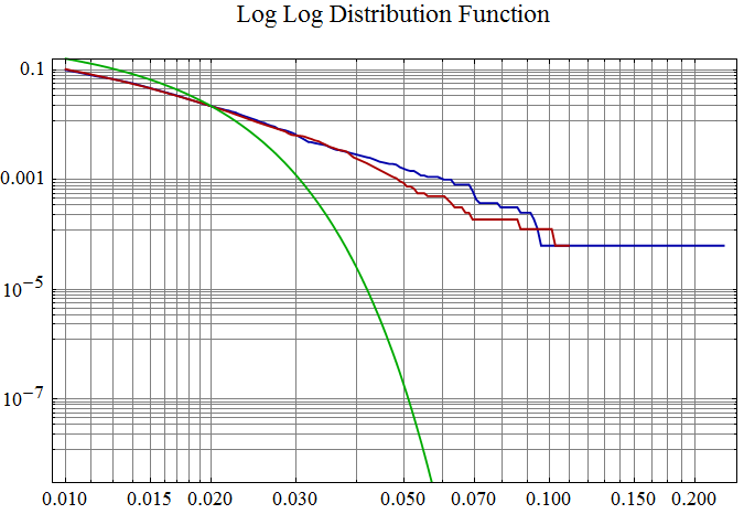
Stable distributions have been suggested as model for financial prices, because they can model heavy Pareto tails and they have the property that they arise as the limiting distribution of sums of identically distributed independent random variables. The rationale for their use is that the longer term log returns could result from the sums of many very small random changes.
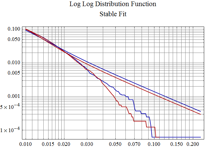
The graph below is similar to the above, but shows a stable fit, with the left tail in blue and the right tail in red. The stable tail fits are the smooth lines while the empirical distribution tails are in the same colors but have jagged lines. The stable tails are significantly heavier than the data tails; consequently the stable distribution will greatly over estimate extreme events. The data tails break away from the stable tails before the p = {0.01, 0.99} level, so a stable distribution would give a more extreme tail event negatively or positively each more than 1% of the time.
Measuring the Financial Log Return Tail Exponent
The plot below is a Mathematica QuantilePlot of the logarithm upper one percent of the right tail data points versus an exponential distribution with the distribution parameter set to one. The idea here is that the log of an Pareto random variable will become an exponential random variable. The reciprocal of the slope, compared to the exponential distribution with λ = 1, gives the tail exponent α, for the Pareto tail. For this to work, the fit must be linear compared to the data, so the graph shows the quality of the fit. Below the graph is the ANOVA Table for the fit and the R Squared value, which would be 1, in the case of a perfect fit.
![Graphics:Quantile Plot Log Right Tail Data vs. ExponentialDistribution[1]](HTMLFiles/MarketReturnDistribution_6.gif)
| DF | SS | MS | F-Statistic | P-Value | |
| t | 1 | 11.1023 | 11.1023 | 11964.2 | 7.86381*10^^-151 |
| Error | 158 | 0.146618 | 0.00092796 | ||
| Total | 159 | 11.2489 |
Below is the quantile/exponential fit to the log of the negative of the lowest 1 % of the log returns to calculate tail exponent of the left tail of the log return distribution.
![Graphics:Quantile Plot Log Left Tail Data vs. ExponentialDistribution[1]](HTMLFiles/MarketReturnDistribution_7.gif)
| DF | SS | MS | F-Statistic | P-Value | |
| t | 1 | 18.2284 | 18.2284 | 10102.4 | 4.1405*10^^-145 |
| Error | 158 | 0.285088 | 0.00180435 | ||
| Total | 159 | 18.5134 |
Both tails are consistent with Pareto tail behavior, with a tail exponent well above the stable regime. Thus the shape of the distribution of financial log returns shows high kurtosis and Pareto like power tails, but the tail behavior, while far heavier that of a normal distribution, has a tail exponent well above that seen for stable distributions. Consequently a stable distribution by virtue of its heavier tails cannot fit the more extreme behavior of market returns, tending to over estimate the magnitudes of the extreme log returns.
Serial Dependence
Another thing to keep in mind when modelling financial data, is that log returns, show serial dependence with respect to their magnitude. This can be demonstrated by looking at the autocorrelation function for the absolute value of log returns, which in this long series shows positive correlation out to 500 market days or about two years. The raw log returns show no apparent structure. This phenomenon is related to the apparent clustering of log returns. It appears that financial data do not have a stationary distribution, but rather could be modeled as a distribution with a varying scale parameter. This scale factor changes slowly so it is often possible to look at epochs of data as if they belong to the same distribution. But the shape of a current distribution may be quite different from a long time series like the one shown on this page.
![Graphics:Autocorrelation Raw Log Returns - Blue Abs[Log Returns] - Red](HTMLFiles/MarketReturnDistribution_8.gif)
© Copyright 2013 Robert H. Rimmer, Jr. Sun 27 Oct 2013