A Market Thought Experiment
A thought experiment to explain the origin of power-tail behavior found in stock market logarithmic returns.
A remarkable finding for stock market price time-series is their consistent, fractal-like appearance over time frames as long as a century. That this persists despite the extraordinary changes in technology used in markets and communications is amazing and suggests an interesting interaction between human behavior and the operation of the continuous double auction market structure. Even though perhaps most trading today is driven by computer programs (written by humans), the fractal-like appearance does not appear to have changed over the past several decades of the technology revolution. To explain some of this behavior we will try a thought experiment.
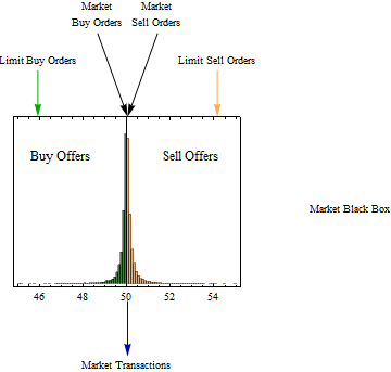
Imagine a market where traders can buy and sell securities, by placing offers to buy or sell at a specific price. Other participants can place orders to buy or sell at the market price, in which case buyers will get the best sell offer, and sellers will get the best buy offer.
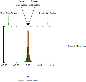
If we take a snapshot of the offered prices at a given time, we might get a picture like shown above. If we made a movie of a sequence of snapshots, we would see all the prices shifting around rapidly. If we blew up any snapshot, we would see a small gap between the best buy offer and the best sell offer. We could change the scaling so that the geometric mean of the best offers is taken as the market price and all other prices are represented as the logarithm of the ratio of each price to the market price. Then our graph would be centered at zero, and if we collected a sequence of snapshots and played them as a movie, we would see the center of the histogram and the heights of the bars would dance up and down, but each frame would be rather similar and we could merge a series of frames for better statistics and study the distribution of logarithmic changes.
There is an interesting paper by Ilija Zovko and J Doyne Farmer, published in 2002, which carefully examines the order books of the London Stock Exchange, between August 1998 and April 2000. The last paragraph of the conclusion is quoted below.
Our results here are interesting for their own sake in terms
of human psychology. They show how a striking regularity can
emerge when human beings are confronted with a complicated
decision problem. Why should the distribution of relative limit
prices be a power law, and why should it decay with this particular
exponent? Our results suggest that the volatility leads the
relative limit price, indicating that traders probably use volatility
as a signal when placing orders. This supports the obvious
hypothesis that traders are reasonably aware of the volatility
distribution when placing orders, an effect that may contribute
to the phenomenon of clustered volatility. Plerou et al (1999)
have observed a power law for the unconditional distribution
of price fluctuations. It seems that the power law for price
fluctuations should be related to that of relative limit prices,
but the precise nature and the cause of this relationship is not
clear. The exponent for price fluctuations of individual companies
reported by Plerou et al is roughly 3, but the exponent we
have measured here is roughly 1.5. Why these particular exponents?
Makoto Nirei has suggested that if traders have power law
utility functions, under the assumption that they optimize
this utility, it is possible to derive an expression for β in terms
of the exponent of price fluctuations and the coefficient of risk
aversion. However, this explanation is not fully satisfying, and
more work is needed. At this point the underlying cause of the
power law behaviour of relative limit prices remains a mystery.
In what follows I will propose a hypothesis to unravel that mystery. I have included a link to the Plerou paper as well because it is the first detailed study of this kind and the results can be reproduced in current markets, so it has stood the test of time. In the Farmer paper above, β is the tail exponent which we will call α. They examined price distances as ticks which were in pence, rather than log returns, but since the tick size is small relative to the price, this will make no difference, and in the process of merging their data sets for different stocks, these distances probably relativized like log returns.
In order to analyze the problem, let’s imagine a trade server that collects a data set for us of all the information coming into the server according to the following algorithm.
First all prices are converted to log prices.
As orders come in they are divided into round lots so one event will be assigned to each 100 shares.
If a market sell order arrives it is executed at the best bid offer and zero is recorded.
If a limit ask order comes in, the best bid offer is subtracted from the mean of the best bid and ask log prices; if the result ≤ 0, the order is executed at the bid price and 0 is recorded, otherwise the difference is recorded as a positive log return.
If a market buy order arrives, it is executed at the best ask offer and zero is recorded.
If a limit bid order comes in, the best ask price is subtracted from the mean of the best bid and ask log prices; if the result is ≥ 0, 0 is recorded and the order is executed, otherwise, the result is recorded as a negative log return.
At each slice of time the resulting data set represents a set of log return distances from the geometric mean of the best bid and ask prices. If this price is also recorded, the actual prices including the spread can be reconstructed.
The server then stores for analysis the sequence of log returns and their arrival times. That some of the limit prices will be later withdrawn is not important here, since we are interested in a snapshot of the price formation process at the instant during which they are present.
I propose the following method of analysis to arrive at a distribution which reflects the process of price formation. First partition the sequence into blocks (it may need to be scrambled at a higher block size if large orders are creating runs of events resulting in a dependent structure). The size of each block should be equal and large enough so that no block contains all zeros, reflecting only transacted prices. It is imagined that the block size will also be significantly larger than this minimum so that we will approach a limiting distribution when we take the next step which is to sum the log returns in each block to create a random variable.
Note I used the term random variable. The idea is that the server has no control over the order the events as they arrive and in market with price execution occurring, there should be an unpredictable flow of market and limit order requests into the server, but this random arrival might need to be ensured by scrambling the order of events. We will now add another assumption, and that is that these log returns will follow a fixed power law as described in Farmer’s paper, for the example we will assume α = 1.5 as was found in the study. Note also that when we sum each block, all the zeros conveniently disappear and have no effect on the result, which effectively becomes a sum of the log returns caused by the limit orders. This sum may accidentally equal zero, but because we have set the block size large enough that it never contains all zeros, the result will not be caused by the executed orders. The block size will affect the scale factor of the distribution, but not the shape of the resulting distribution. Since we may want to have a convenient interpretation of the scale factor, we might want to select a block size as the average number of events that arrive in a specific time unit, perhaps a second for actively traded stocks or a minute for less active trading.
What we have imagined is a sum of independent identically distributed random variables from a heavy-tailed distribution. By pure mathematics of the generalized central limit theorem we know that the limiting distribution of these sums will be a stable distribution with tail exponent, α = 1.5; it will have a skewness parameter, β, which depends upon the balance of returns above and below the mean. The scale factor, γ, will depend on our block size or the number of events and the data histogram, and itself will scale by γ n^(1/α), where n is the block size. Finally, the parameter, δ, will represent the mean or expectation of our collection of random variables. It is also possible for the bid and ask tail exponents to be different and still have convergence to a limiting stable distribution, in that case the α of the limiting stable distribution will have the α of the lower tail exponent. All of the statements in this paragraph are true if the random variable source is i.i.d.
What we have done in our thought experiment above is to create a distribution which in a fashion describes the process of price formation. We have used log returns to have relative price changes rather than actual prices, but if the central price were known we could calculate actual prices over some window related to the size of the data block. The next step is to solve the riddle of the higher tail exponent in transacted prices. The first problem we have is that the distribution we have created does not tell us which return events would result in transactions and we have complicated the analysis by summing the data stream. But let’s consider that the process we are describing will portray the spectrum of prices which could be transacted over a window consistent with our block size; then the log returns of executed prices might be similar to a subset of this price formation distribution.
How do we find that subset? First there is a symmetry in every transaction, it requires both a buyer and a seller. So we make the assumption that traders who place limit orders have some expectation that prices they set could be executed, but they have also set some prices that they expect to have very low probability of execution, and in fact most of these orders may never be executed. Next we assume that the expectations for execution of an order should be symmetric on the bid and ask sides. Suppose that the expectations are such that the middle third of the distribution is most likely to be executed. Then we could extract the distribution of log returns which should be executed by order statistics. To do this we generate a set of random three variables from our stable price formation distribution. We sort the three values, select the median value and discard the other two. A set of random variables collected in this way has a known distribution which can be calculated from the parent stable distribution; it is the 2:3 order statistic distribution of the parent stable distribution. The formula for the density of this distribution is below.
![]()
where f(x) is the density of the parent distribution and F(x) is the parent distribution function.
A graph of three order statistic distributions derived from a stable distribution with parameters {α, β, γ, δ} = {1.5, 0.3, 1, 0} is shown below. The parent distribution is in blue and the densities of the order statistic distribution are scaled by one third, since the sum of these scaled densities would equal the parent density. The red curve is the 1:3 order statistic density, the yellow is the 2:3 density we are interested in, and the green is the 1:3 density.
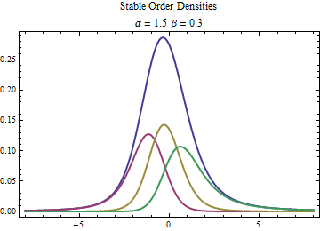
The 2:3 order statistic distribution has the interesting property that its tail exponent will be exactly twice that of the parent distribution. Thus it will have the desired tail exponent of 3 if we start with a parent stable distribution having α = 1.5. It will have three other parameters, β, representing skewness, γ representing scale, and δ representing location, but these parameters will have different interpretation than they would for the parent stable distribution. For instance, δ will only represent the expectation in the case of a symmetric distribution, where β = 0.
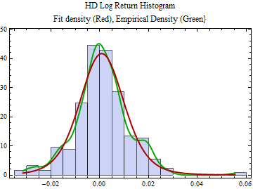
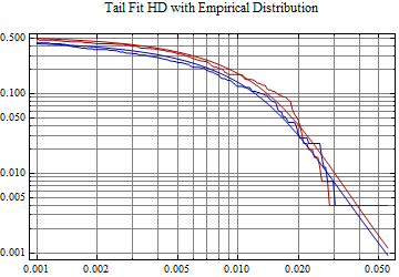
I have developed Mathematica code to fit the stable 2:3 order statistic distribution and below is fit to the most recent year’s data for INTC. The fit density is in red, the smoothed empirical density is in green. The tail fit shows the log log plots of the distribution function: CDF[-x], the left tail, in blue, and 1-CDF[x], the right tail, in red. The x-axis is Abs[x], and the y-axis is probability for the left tail and 1 - probability for the right tail.
Mathematica users may download the notebook and try fits to many different stocks. This notebook does not include the fitting code which is in S23Distribution.nb and must be executed first.
It should be possible to turn this thought experiment into a real experiment with a good quality data feed providing level II quotes. The algorithm would have to be changed to ensure the structure was represented properly; this could perhaps be done with histogram data snapshots to create the random variable stream. If anyone tries this, please let me know. I would also be happy to help with the algorithm and analysis. Bob Rimmer
An interactive module which requires Wolfram CDF Player or Mathematica to be installed on the computer shows the stable 2:3 order statistic density and distribution functions and allows the parameters to be changed.
Stable 2:3 Order Statistic Distribution
© Copyright 2013 Robert H. Rimmer, Jr. Fri 1 Nov 2013