S23Test
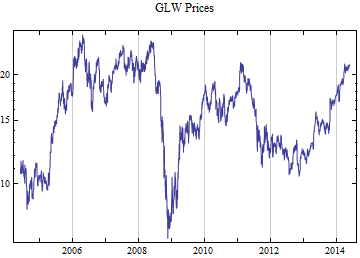
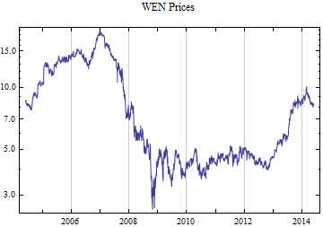
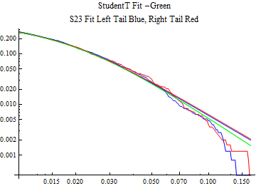
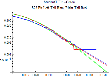
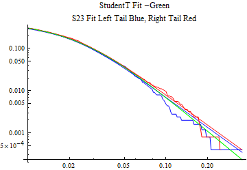
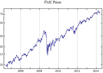
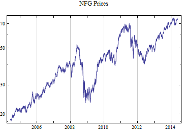
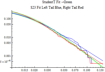
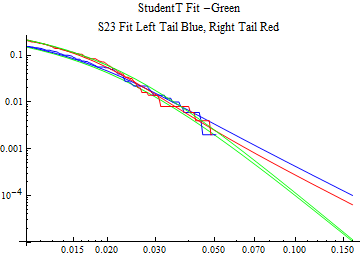
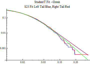
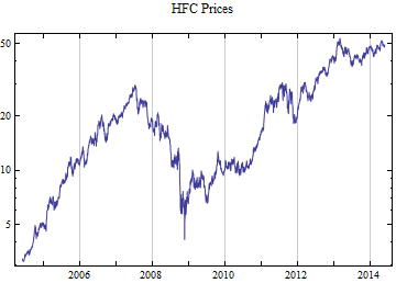
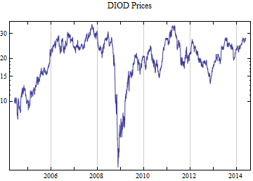
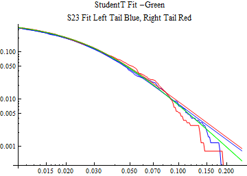
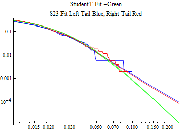
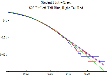
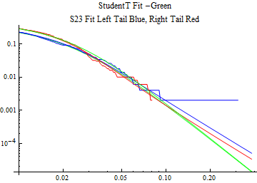
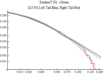
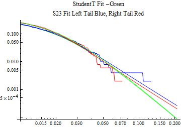
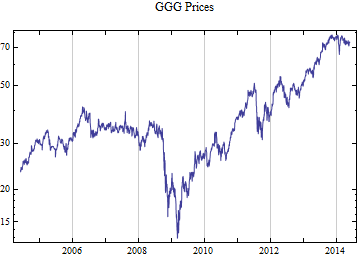
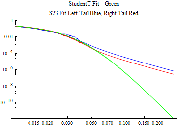
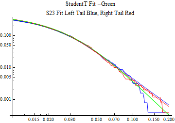
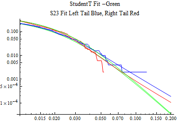
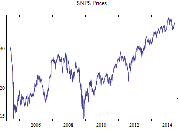
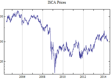
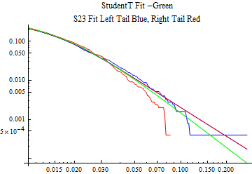
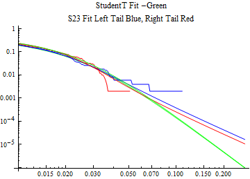
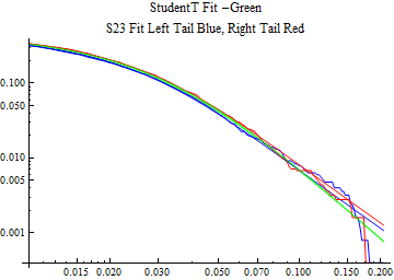
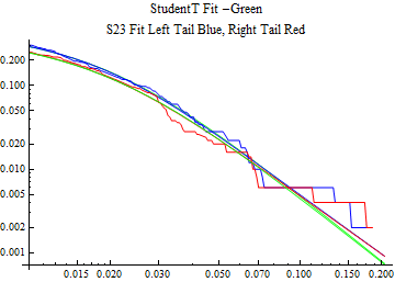
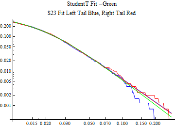
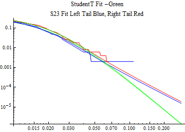
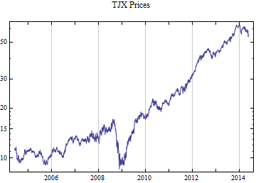
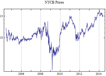
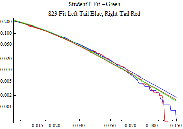
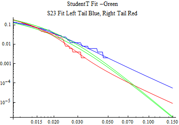
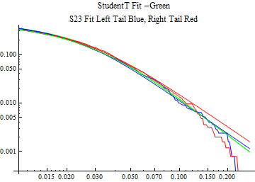
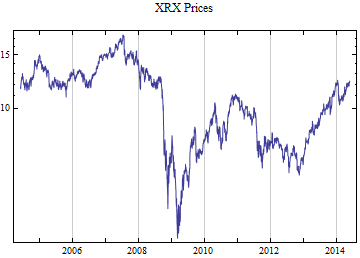
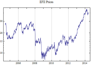
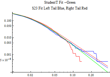
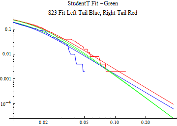
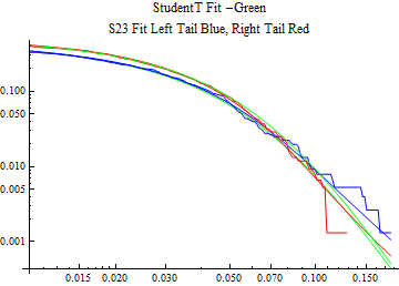
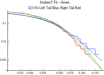
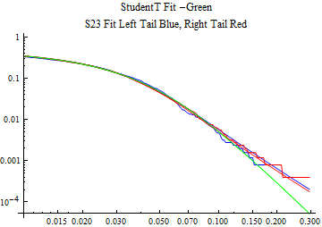
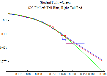
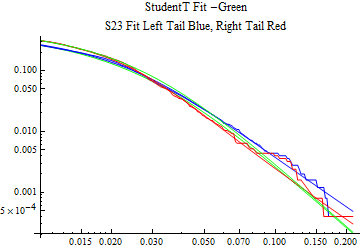
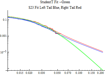
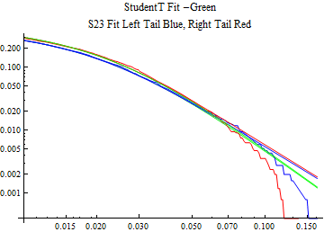
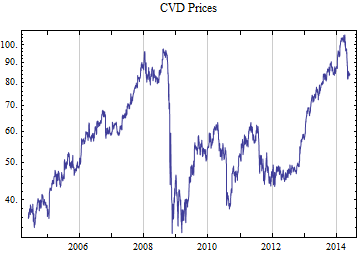
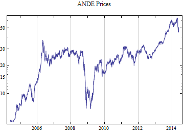
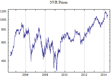
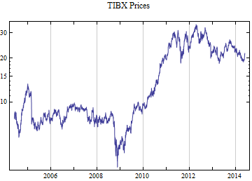
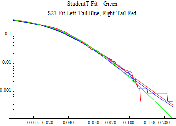
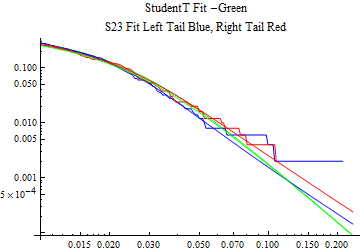
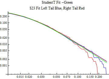
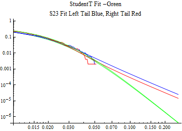
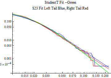
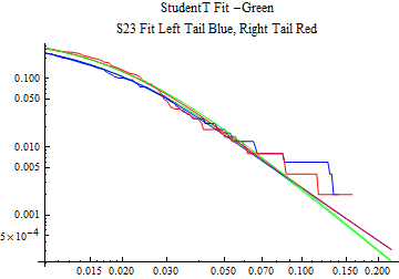
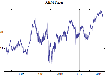
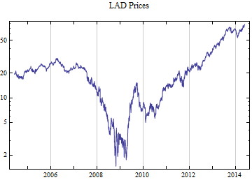
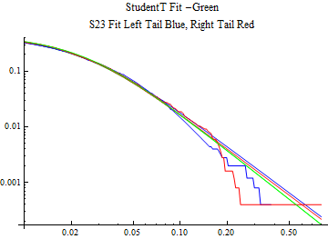
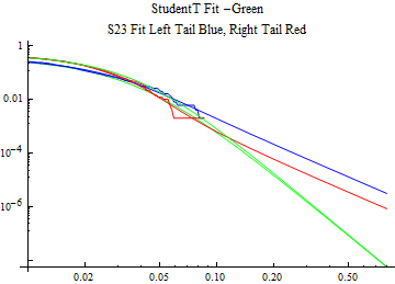
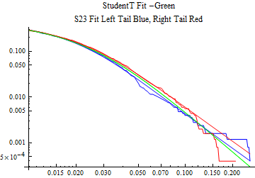
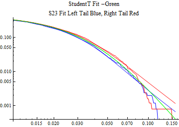
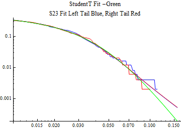
How good is the stable 2:3 order statistic distribution as a model for financial data, compared to the Student T distribution which can also model heavy tailed behavior? This notebook selects at random 50 ticker symbols which have more than ten years of daily data from the S&P 1500 constituent list. The last decade of data presents an interesting challenge in that it has the highest volatility since the Great Depression as well as some of the lowest volatility ever recorded. To capture both aspects of the data set. Each distribution was fit to the whole ten years of daily logarithmic returns and the most recent 500 returns, when the volatility was significantly lower. Maximum likelihood fitting was used for both models. This method tends to give the most accurate fit, but the fit to the tail behavior particularly in small samples depends upon having the best model. There are not good numerical methods to assess the tail fit so it is done graphically, comparing the empirical data distributions to the model fits. The restriction to a limit of 500 data points should limit the data to no more than 5 points on each tail beyond the p = 0.01 level, thus presenting a significant challenge to get the tail behavior right.
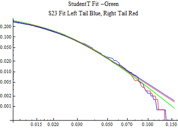
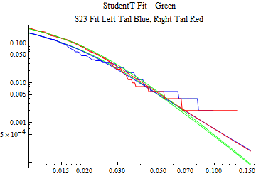
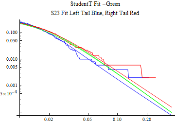
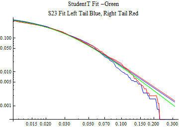
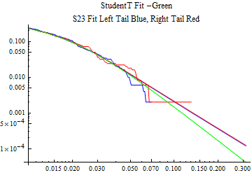
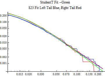
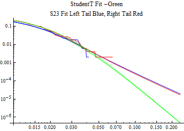
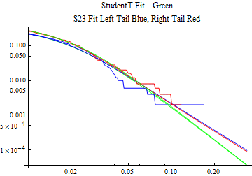
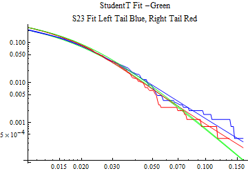
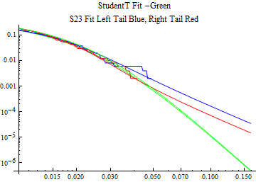
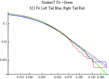
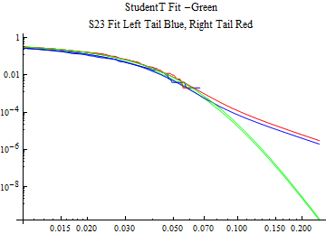
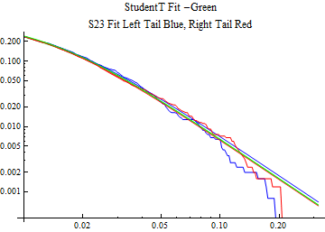
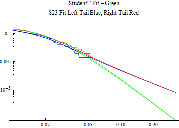
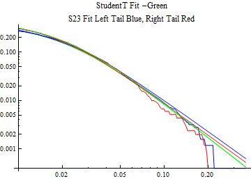
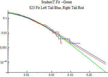
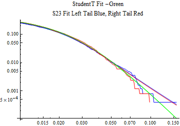
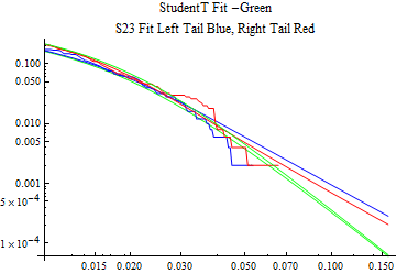
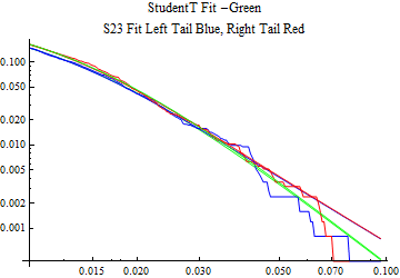
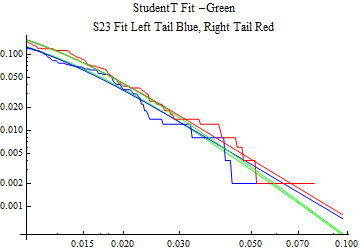
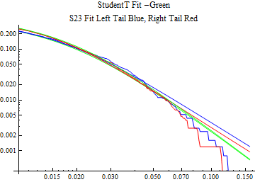
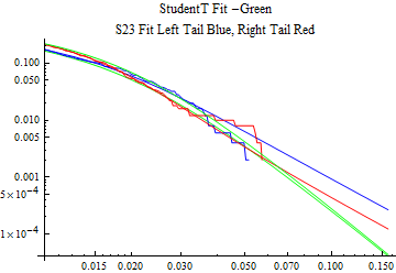
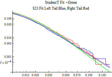
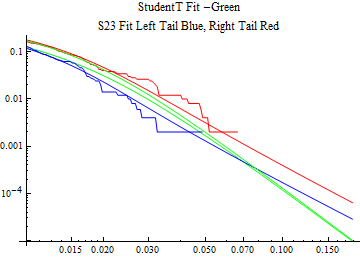
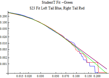
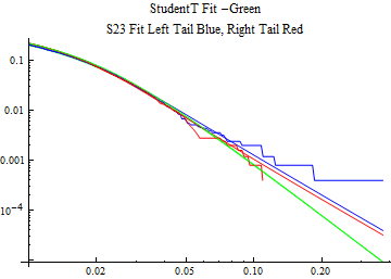
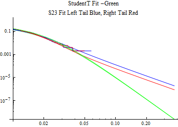
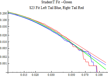
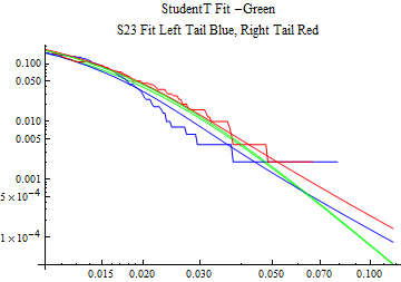
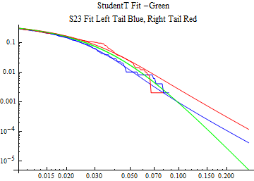
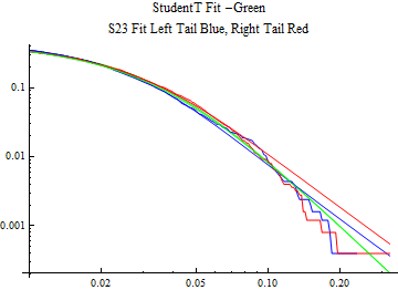
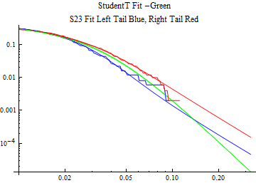
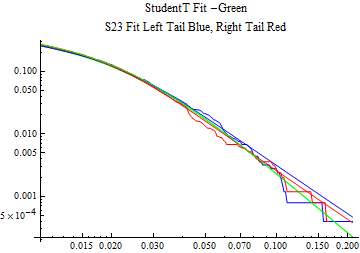
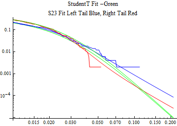
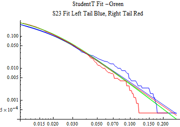
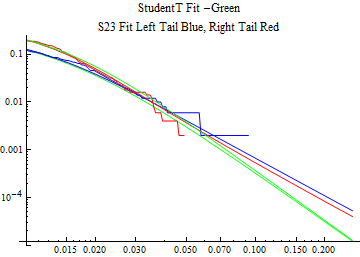
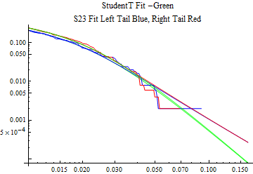
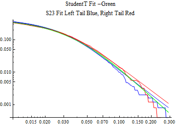
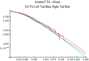
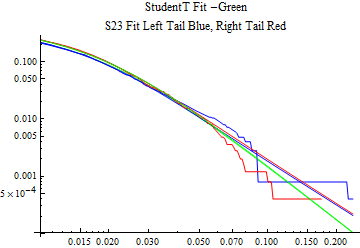
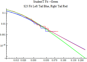
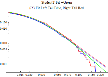
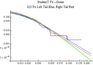
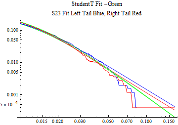
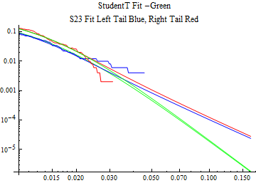
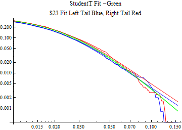
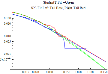
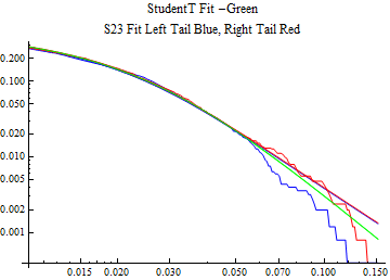
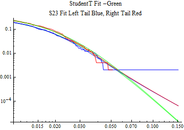
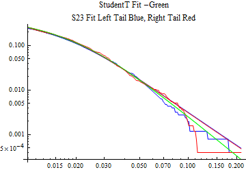
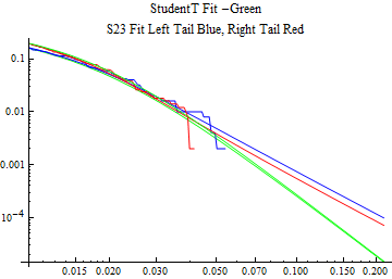
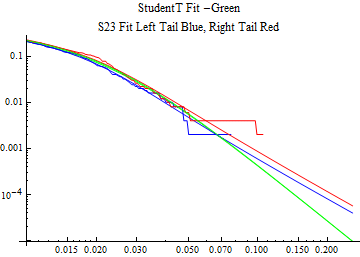
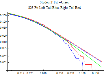
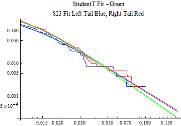
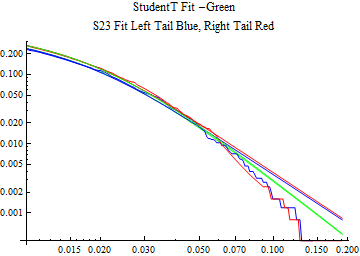
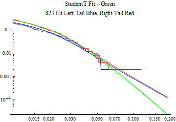
The fits are shown in the form StudentTDistribution[ μ, σ, ν] where μ is the location parameter, σ is the scale parameter and ν is the shape parameter. For the stable 2:3 order statistic distribution the parameters are shown as S23OrderDistribution[ α, β, γ, δ ] where α is the tail parameter, double that of the parent stable distribution and β, γ, δ, correspond respectively to the skewness parameter, scale parameter, and location parameter of the parent stable distribution. The tails are plotted on a log log plot with 1- probability for the right tail in red and the probability for the left tail in blue against the magnitude of x. The tails of the Student T distribution are shown in a single color green, since this is a symmetric distribution, they will converge, whereas for the stable 2:3 order distribution there will be parallel power tails if β is not close to zero. The empirical distribution has the same red and blue tail colors but has the jagged curve since each point is essentially a discrete event.
On the graphs both tails are represented as negative slopes. The steeper slopes have the lighter tail behavior and the more horizontal slopes have the heavier tail behavior.
The software notebook used below can be found here: http://pages.suddenlink.net/rhr/s23/S23Distribution.nb
NotebookEvaluate["C:\\Mathematica 9\\MarketModel2013\\S23\\S23Distribution.nb"];
tickerList = {"GLW", "WEN", "MW", "NANO", "FMC", "NFG", "TBI", "CKH", "HFC", "DIOD", "PLXS", "CVGW", "BK", "MYE", "TXN", "MDLZ", "GGG", "MCK", "NPBC", "GVA", "SNPS", "ISCA", "EZPW", "EAT", "TJX", "NYCB", "LEN", "DHI", "XRX", "EFII", "DDD", "ATML", "OCR", "NBL", "BKE", "KLIC", "CVD", "ANDE", "WM", "GWR", "NVR", "TIBX", "BBCN", "HPQ", "ABM", "LAD", "SYKE", "UNF", "EMN", "RGLD"};
startDate = DatePlus[Take[DateList[], 3], {-10, "Year"}]
Do[data = FinancialData[tickerList[[i]], startDate];
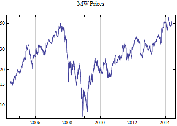
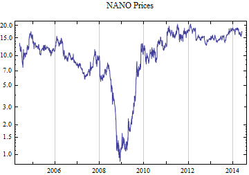
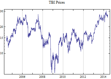
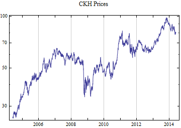
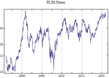
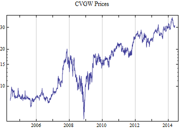
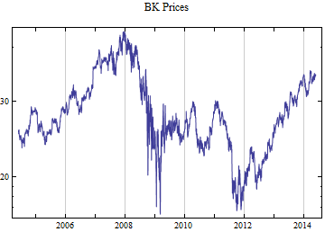
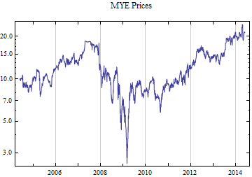
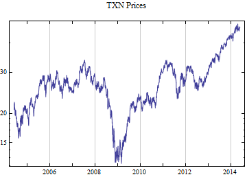
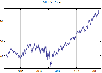
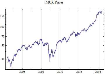
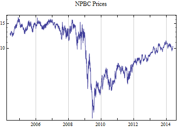
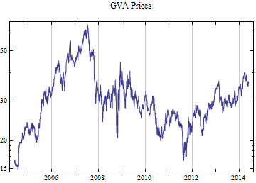
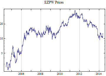
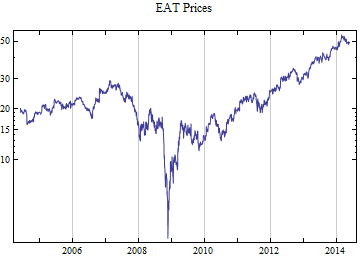
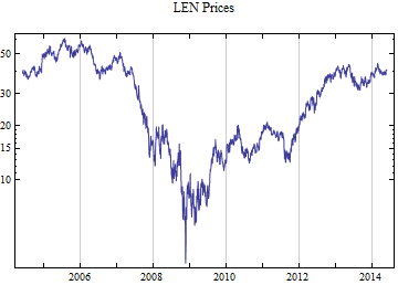
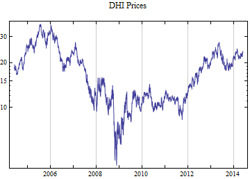
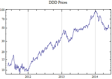
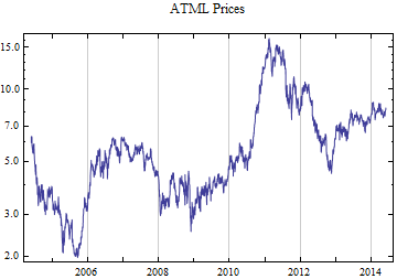
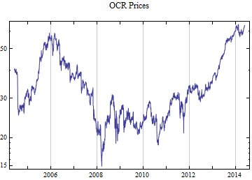
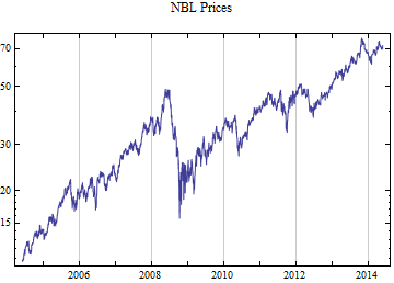
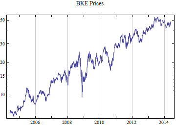
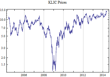
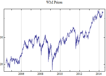
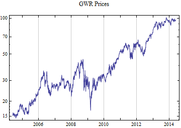
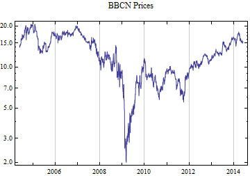
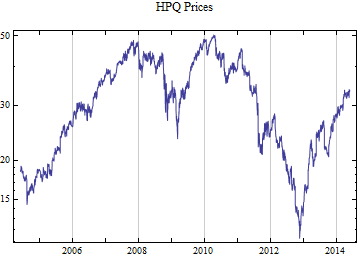
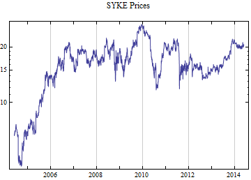
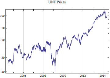
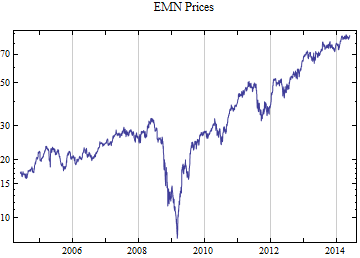
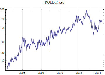
Print[DateListLogPlot[data, Joined -> True, PlotRange -> All, PlotLabel -> tickerList[[i]] <> " Prices"]];
lr = Differences[Log[data[[All, 2]]]];
max = Max[Abs[lr]];
std = EstimatedDistribution[lr, StudentTDistribution[μ, σ, ν]];
s23 = Quiet@S23MLFit[lr, {3, 0, 0.01, 0}];
empD = EmpiricalDistribution[lr];
Print["Ten Year Fit Parameters"];
Print[std];
Print["S23OrderDistribution[" <> StringReplace[ToString[s23, StandardForm], {"{" -> "", "}" -> ""}] <> "]"];
Print[LogLogPlot[{CDF[std, -x], CDF[S23OrderDistribution[s23], -x], CDF[empD, -x], 1 - CDF[S23OrderDistribution[s23], x], 1 - CDF[empD, x], 1 - CDF[std, x]}, {x, 0.01, max}, PerformanceGoal -> "Speed", PlotStyle -> {Green, Blue, Blue, Red, Red, Green}, PlotLabel -> "StudentT Fit -Green\nS23 Fit Left Tail Blue, Right Tail Red"]];
lr = Take[lr, -500];
std = EstimatedDistribution[lr, StudentTDistribution[μ, σ, ν]];
s23 = Quiet@S23MLFit[lr, {3, 0, 0.01, 0}];
empD = EmpiricalDistribution[lr];
Print["Two Year Fit Parameters"];
Print[std];
Print["S23OrderDistribution[" <> StringReplace[ToString[s23, StandardForm], {"{" -> "", "}" -> ""}] <> "]"];
Print[LogLogPlot[{CDF[std, -x], CDF[S23OrderDistribution[s23], -x], CDF[empD, -x], 1 - CDF[S23OrderDistribution[s23], x], 1 - CDF[empD, x], 1 - CDF[std, x]}, {x, 0.01, max}, PerformanceGoal -> "Speed", PlotStyle -> {Green, Blue, Blue, Red, Red, Green}, PlotLabel -> "StudentT Fit -Green\nS23 Fit Left Tail Blue, Right Tail Red"]];
Print["**********************************************"];
Print[],
{i, Length[tickerList]}] // AbsoluteTiming
![]()
![]()
![]()
![]()
![]()
![]()
![]()
![]()
![]()
![]()
![]()
![]()
![]()
![]()
![]()
![]()
![]()
![]()
![]()
![]()
![]()
![]()
![]()
![]()
![]()
![]()
![]()
![]()
![]()
![]()
![]()
![]()
![]()
![]()
![]()
![]()
![]()
![]()
![]()
![]()
![]()
![]()
![]()
![]()
![]()
![]()
![]()
![]()
![]()
![]()
![]()
![]()
![]()
![]()
![]()
![]()
![]()
![]()
![]()
![]()
![]()
![]()
![]()
![]()
![]()
![]()
![]()
![]()
![]()
![]()
![]()
![]()
![]()
![]()
![]()
![]()
![]()
![]()
![]()
![]()
![]()
![]()
![]()
![]()
![]()
![]()
![]()
![]()
![]()
![]()
![]()
![]()
![]()
![]()
![]()
![]()
![]()
![]()
![]()
![]()
![]()
![]()
![]()
![]()
![]()
![]()
![]()
![]()
![]()
![]()
![]()
![]()
![]()
![]()
![]()
![]()
![]()
![]()
![]()
![]()
![]()
![]()
![]()
![]()
![]()
![]()
![]()
![]()
![]()
![]()
![]()
![]()
![]()
![]()
![]()
![]()
![]()
![]()
![]()
![]()
![]()
![]()
![]()
![]()
![]()
![]()
![]()
![]()
![]()
![]()
![]()
![]()
![]()
![]()
![]()
![]()
![]()
![]()
![]()
![]()
![]()
![]()
![]()
![]()
![]()
![]()
![]()
![]()
![]()
![]()
![]()
![]()
![]()
![]()
![]()
![]()
![]()
![]()
![]()
![]()
![]()
![]()
![]()
![]()
![]()
![]()
![]()
![]()
![]()
![]()
![]()
![]()
![]()
![]()
![]()
![]()
![]()
![]()
![]()
![]()
![]()
![]()
![]()
![]()
![]()
![]()
![]()
![]()
![]()
![]()
![]()
![]()
![]()
![]()
![]()
![]()
![]()
![]()
![]()
![]()
![]()
![]()
![]()
![]()
![]()
![]()
![]()
![]()
![]()
![]()
![]()
![]()
![]()
![]()
![]()
![]()
![]()
![]()
![]()
![]()
![]()
![]()
![]()
![]()
![]()
![]()
![]()
![]()
![]()
![]()
![]()
![]()
![]()
![]()
![]()
![]()
![]()
![]()
![]()
![]()
![]()
![]()
![]()
![]()
![]()
![]()
![]()
![]()
![]()
![]()
![]()
![]()
![]()
![]()
![]()
![]()
![]()
![]()
![]()
![]()
![]()
![]()
![]()
![]()
![]()
![]()
![]()
![]()
![]()
![]()
![]()
![]()
![]()
![]()
![]()
![]()
![]()
![]()
![]()
![]()
![]()
![]()
![]()
![]()
![]()
![]()
![]()
![]()
![]()
![]()
![]()
![]()
![]()
![]()
![]()
![]()
![]()
![]()
![]()
![]()
![]()
![]()
![]()
![]()
![]()
![]()
![]()
![]()
![]()
![]()
![]()
![]()
![]()
![]()
![]()
![]()
![]()
![]()
![]()
![]()
![]()
![]()
![]()
![]()
![]()
![]()
![]()
![]()
![]()
![]()
![]()
![]()
![]()
![]()
![]()
![]()
![]()
![]()
![]()
![]()
![]()
![]()
![]()
![]()
![]()
![]()
![]()
![]()
![]()
![]()
![]()
![]()
![]()
![]()
![]()
![]()
![]()
![]()
![]()
![]()
![]()
![]()
![]()
![]()
![]()
![]()
![]()
![]()
![]()
![]()
![]()
![]()
![]()
![]()
![]()
![]()
![]()
![]()
![]()
![]()
![]()
![]()
© Copyright 2014 Robert H. Rimmer, Jr. Fri 30 May 2014