Stable Fit to Rescaled Data
This is an in depth look at a non-stationary model of a stable distribution with varying scale factor, which has serial dependence.
This notebook develops an approach to fitting distribution by adjusting the data. In general modifying data is a bad idea, especially when the assumptions are not known to be true, so these methods are not recommended for fitting financial data. The goal rather is to look at how well the idea performs, before pursuing other methods such as a mixture distribution. The hypothesis is to consider the possibility that the underlying market distribution is a stable distribution with a scale factor, γ, which varies every day, and attempt to modify the data to standardize the scale. The time-series is the same that is demonstrated in detail in MarketReturnDistribution.
Start ... Tuesday 3 January 1950
End ... Friday 25 October 2013
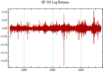
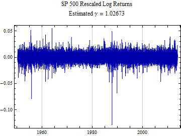
Below is a graph of the daily changes in log returns for the S&P 500 series since 1950. Epochs of high and low volatility tend to cluster together. The strategy is to use this dependent structure to determine the scale factor for the data in small blocks; in this case the time-series is divided into 63 market day or about 3 month blocks.

What is needed next is a reasonably accurate method to estimate the stable scale factor on a small sample. There is a method based on the stable characteristic function which is independent of other parameters. It is outlined below.
The stable characteristic function, φ, may be written in polar coordinate form, ![]() .
.
![]()
The absolute value of the characteristic function, |φ(t)|, the r factor, is the symmetric strictly stable characteristic function, where β = 0 and δ = 0.
![]()
The characteristic function can be approximated from a data sample, using the formula for the empirical characteristic function, ecf, where ![]() , {k ∈ {1, ..., n}, are the sample random variables.
, {k ∈ {1, ..., n}, are the sample random variables.

Equation (2) offers the possibility of quickly approximating γ at the point t = 1, by scaling the set of random variables so that γ = 1 and the characteristic function at this point = ![]() . Equation (4) may be solved numerically for γ.
. Equation (4) may be solved numerically for γ.

The method is less accurate than maximum likelihood fitting, but the methods are comparably bad for small sample sizes. The idea is that the method doesn’t have to be too precise, because the day to day variation in the magnitude of the log returns is large.
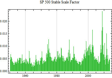
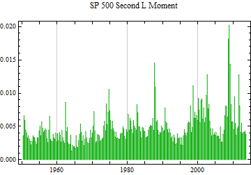
The variation in the method is also comparable to another method of measuring scale, the second L Moment. The stable scale factor, γ, can be derived from the second L Moment, ![]() by the following linear relationship.
by the following linear relationship.

This relationship requires the assumption that the tail exponent, α, of the stable distribution remains stationary, but also can serve to substantiate the accuracy of the method, although neither method could be considered a gold standard for measuring the scale factor of a stable distribution over a small sample size.
The graph below shows the linear regression between the two methods for determining a stable scale factor.
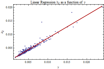
From the slope of the fit with the assumption that α is stationary, we can derive and estimate for α.
![]()
The ANOVA table and the RSquared calculation from the linear regression are below.
| DF | SS | MS | F-Statistic | P-Value | |
| x | 1 | 0.00139175 | 0.00139175 | 2802.44 | 1.56467*10^^-138 |
| Error | 252 | 0.000125148 | 4.96619*10^^-7 | ||
| Total | 253 | 0.00151689 |
The graph below shows the rescaled returns, which were derived by dividing each block of returns by the estimated scale factor for that block. This division should have the effect of bringing the scale factor, γ, of the adjusted returns to 1.0.
The autocorrelation functions of the absolute value of the raw returns and the absolute value of the rescaled returns shows that most of the serial dependence has been eliminated by the rescaling.
![Graphics:Autocorrelation Raw Abs[Returns] - Red Abs[Rescaled Returns] - Blue](HTMLFiles/RescaledStableFit_16.gif)
The log log plot of the tail fit shows that a stable fit to the rescaled returns still has a heavier tail in the data, but the tails break away further out on each tail.
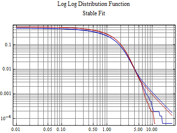
It can be seen that the fit of the rescaled data is much better on the tails and α is considerably higher than the fit to the same data in the MarketReturnDistribution notebook. Ultimately, however, rescaling the data does not change the extreme tail behavior of a data set. The extreme tail is still lighter than the stable fit, with the fit tail breaking away from the data tails at the p = {0.004, 0.996} tail level, so a large central part of the distribution is better fit by a stable distribution.
The charts below estimate the tail exponents for the rescaled log returns using the same method shown in MarketReturnDistribution notebook. And α is still well above the stable regime.
![Graphics:Quantile Plot Log Right Tail Data vs. ExponentialDistribution[1]](HTMLFiles/RescaledStableFit_18.gif)
| DF | SS | MS | F-Statistic | P-Value | |
| t | 1 | 11.1023 | 11.1023 | 11964.2 | 7.86381*10^^-151 |
| Error | 158 | 0.146618 | 0.00092796 | ||
| Total | 159 | 11.2489 |
![Graphics:Quantile Plot Log Left Tail Data vs. ExponentialDistribution[1]](HTMLFiles/RescaledStableFit_19.gif)
| DF | SS | MS | F-Statistic | P-Value | |
| t | 1 | 11.9174 | 11.9174 | 6272.49 | 4.46554*10^^-129 |
| Error | 158 | 0.300193 | 0.00189995 | ||
| Total | 159 | 12.2176 |
What does all this mean? Probably not very much, but it seems clear that rescaling the data does not eliminate distal power tail behavior which is lighter than supported by a stable distribution. The theoretical implications are the most important. Stable distributions evolve from the summation of identically distributed, independent random variables, which have a tail exponent, α < 2. If α ≥ 2, the distribution should have finite variance and the generalized central limit theorem should eventually lead to a normal distribution behavior. The rescaling method did seem to remove the serial dependent structure shown in the autocorrelation of absolute returns.
Consequently the idea that price formation arises from the sums of many very small differences in price or log returns seems not to be probable as this index is currently derived from hundreds of millions of transactions daily. Mathematica users may download the notebook and substitute the log return data for a set of stable random variables multiplied by a slowly varying scale function and demonstrate that the initial stable distribution parameters can indeed be recovered by the methods shown here.
When intraday price data are examined closely a lot more structure is revealed; there is a serial dependent structure which evolves through the day with higher scale factor and volume per minute near the open and close of trading, compared with the transactions in the middle of the day. Yet when the tail behavior of the intraday data is examined, it also shows a power tail structure with a tail exponent, α, greater than 2.
© Copyright 2013 Robert H. Rimmer, Jr. Sun 27 Oct 2013