Treasury Zero Coupon Bonds
A model for the price structure of zero coupon Treasury bonds is based on the survival function of a probability distribution arising from the sum of an exponential distribution random variable and a gamma distribution random variable. The three-parameter function is used to fit prices of zero coupon treasury bonds with respect to their time to maturity with excellent results.
The data are obtained from the Wall Street Journal web page below which lists bid and ask quotes for zero coupon Treasury bonds as of 3 PM ET each day for trades of one million dollars or more. The program imports the data from the page and fits it to the model, which is presented in detail. All the code to reproduce what follows is contained in the notebook.
http://online.wsj.com/mdc/public/page/2_ 3020-tstrips.html
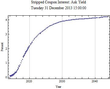
Here is a plot of the average yield to maturity curve versus maturity date provided in the data.

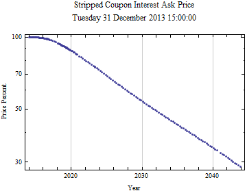
Below is the plot of the ask price versus the maturity date on a logarithmic scale. Note that it is nearly perfectly linear on this plot as time goes on. This suggests a pure exponential model could be used to fit the long term data.
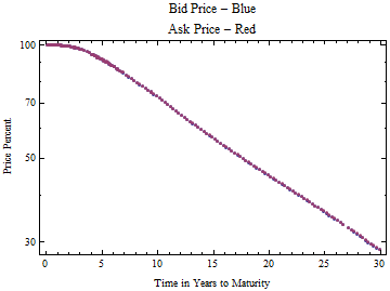
The function can be adjusted from price based on maturity date to price versus time to maturity. In this way the curve can be compared to previous and future curves, as starting at time zero. Plots of both the bid and ask prices are shown below on a log scale plot. Note that the price structures are identical and the linearity suggests a exponential decay model for the longer maturities.
The plots below show ΔLog[price]/Δt, since all the prices should be declining as time to maturity increases, the values (which are essentially annualized log returns) theoretically should be negative. There is a lot of variation in the maturities below 10 years, but the general trend is declining. After 10 to 12 years, the rate of change becomes nearly constant consistent with an exponential decay model.

If the price percent is converted to decimal price, the shape of the curve has the properties of a survival function. A rational assumption is that the price function, p(t) is always decreasing, i.e. the longer an investor has to wait for maturity of a bond, the greater the return he expects. This further requires the first derivative, p’(t) always be negative. The linearity of the distal part of the curve on the log plot is consistent with an exponential decay function:
![]()
where r is the logarithmic rate of return and t is time. This also happens to be the survival function of an exponential distribution with parameter, r. The initial part of the price curve, however, is not at all like an exponential distribution survival function. But it is a little like the survival function of a gamma distribution. A better fit comes from the convolution of the gamma distribution and an exponential distribution; this is the distribution of the sum of an exponential distribution random variable and a gamma distribution random variable.
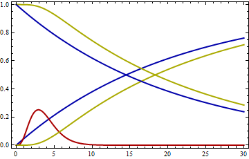
To visualize the convolution process the graph below shows the density of a gamma distribution, in red, convolved with the distribution function of an exponential distribution, the rising blue curve. The result of the convolution is the rising yellow curve. The survival function of the original exponential distribution is the declining blue curve, and the declining yellow curve is the survival function of the convolved distribution, which is our priceModel equation shown below. In fitting the prices we multiply the model by 100 to be consistent with bond prices in percent.

Where Γ is the gamma function.
The plot below shows the model fit in red to the data points on a log scale plot.
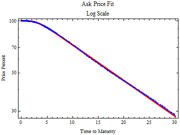
The coefficient of determination is rather good, meaning that all the prices line up with the model well at an instant of time. But the model parameters change significantly with time, even through the course of a day.
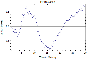
Coefficient of determination, R Squared: 0.999979.The fit residuals are shown below.
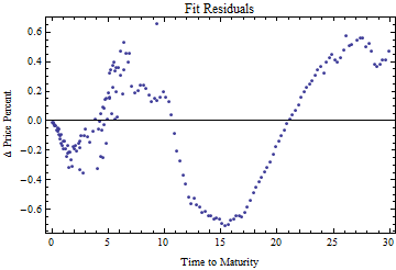
The formula and parameter set for the fit to the ask price are shown below.

![]()
The parameter statistics are below. The dominant rate, r0, from the exponential distribution component, determines the long maturity schedule. The interpretation of the other two parameters is more difficult; they are the parameters from the gamma distribution component. But it should be remembered that a gamma distribution parameterized as in this notebook represents the distribution of the sum of k exponential distribution random variables with parameter, r1. k is not an integer here, but the distribution should be able to represent fractional random variables.
| Estimate | Standard Error | t-Statistic | P-Value | |
| r0 | 0.0474647 | 0.00010392 | 456.742 | 1.58577*10^^-264 |
| r1 | 1.33275 | 0.0985827 | 13.5191 | 9.51599*10^^-29 |
| k | 4.24368 | 0.294596 | 14.4051 | 2.90749*10^^-31 |
The 95% confidence intervals of the parameters are shown below.
| Estimate | Standard Error | Confidence Interval | |
| r0 | 0.0474647 | 0.00010392 | {0.0472596,0.0476699} |
| r1 | 1.33275 | 0.0985827 | {1.13814,1.52735} |
| k | 4.24368 | 0.294596 | {3.66215,4.82522} |
We can create a log price function, take the first derivative negative of that, to create an instantaneous yield curve. This function asymptotically approaches r0.
![Graphics:First Derivative of -Log[askPrice]](HTMLFiles/TreasuryZeroes_12.gif)
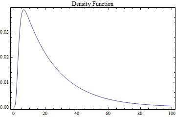
Another interesting feature of the model is that if you divide the price by 100, it is a survival distribution function; if you take the derivative of 1 - SurvivalFunction(.), you get a picture of the underlying probability density function, which integrates to 1 as t goes from 0 → ∞. This appears to be a density of times to maturity, but it is not clear how to interpret this--there isn’t any Treasury debt over 30 years duration. But it would be interesting to compare to the maturity of outstanding available debt, and perhaps compare that to a truncated distribution. It probably should be influenced by the maturities of debt issued by the Treasury and by the Federal Reserve Bank activity of taking securities out of the market place; the Fed now owns more than 17% of the public debt.
The program can also easily be used with data copied from a brokerage account web interface, even though the web security won’t allow you to gather the data directly. Below is a fit obtained from data from set of Schwab Brokerage web pages to obtain a price curve for Treasuries offered on their site on 4 December 2013. Four web pages of data were pasted into a Mathematica string then imported into a table for analysis, using the function, ImportString[]. The full code for the example is included in the down-loadable notebook.

![]()
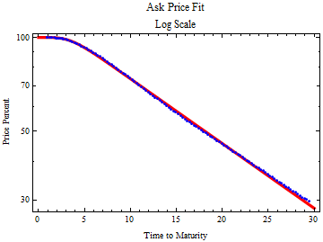
| Estimate | Standard Error | t-Statistic | P-Value | |
| r0 | 0.0479334 | 0.000141185 | 339.508 | 1.94257*10^^-174 |
| r1 | 1.62613 | 0.195678 | 8.31023 | 2.15031*10^^-13 |
| k | 5.79357 | 0.67326 | 8.60526 | 4.52361*10^^-14 |
It may be possible to use this model to study the shape of the pricing structure for all Treasury bonds. Daily Treasury yield curves can be converted to zero coupon prices and fit to the model. It will be interesting to watch how the parameter structure changes as the Federal Reserve withdraws its quantitative easing.
The price curves can also be turned around to look at the expected growth with time for a specific bond. For instance, if you are holding a zero coupon bond, does it make sense to sell it before it matures and buy another one with longer maturity, in order to maximize return, which begins to decline as the bond approaches maturity? When a yield is calculated for a zero coupon bond, it is based on an average yield to maturity, but if you are holding a bond you receive higher yield while the maturity is in the distant future and much lower yield as it approaches maturity.
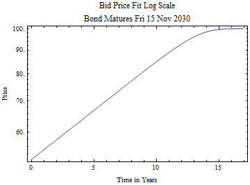
If you paste the code below into a Mathematica notebook and execute it, you will open this notebook into Mathematica and all the code will be available by opening the closed cells.
NotebookPut@Import["http://pages.suddenlink.net/rhr/fin07/TreasuryZeroes.nb"];
There are interactive modules which require Wolfram CDF Player or Mathematica to be installed on the computer. The Zero Coupon Model explores the three-parameter bond yield function and its first two derivatives in detail; the Yield Curve module reconstructs the traditional yield curve from the model.
© Copyright 2014 Robert H. Rimmer, Jr. Thu 2 Jan 2014